From GraphDB Ontologies to Embeddings: Modeling Fuzzy Relationships

#

Keywords: GraphDB, VectorDB, Ontology, Embedding Vectors

I was talking to a friend who uses a graphDB in their AI app and has run into an interesting problem. The quality is low because there are often many terms for the same thing, and many terms with multiple meanings depending on context. For example, if you’re looking for people to go on a walk with, it’s likely that people who like running or hiking are good candidates, but this may not be well represented in your graphDB. There’s a traditional way to solve this and more modern one using a vectorDB (weaviate, postgres with pgvector, etc.).

One approach is to create an ontology around this idea of activities and encode how related they are as a number. For example, if I like running maybe that means there’s an 80% chance I’ll like walking (even though I didn’t say so), and if I like hiking perhaps there’s a 90% chance I’ll like walking. Plus, in the other direction, if I like walking I’m also 90% likely to like hiking.

IMG-SOURCE

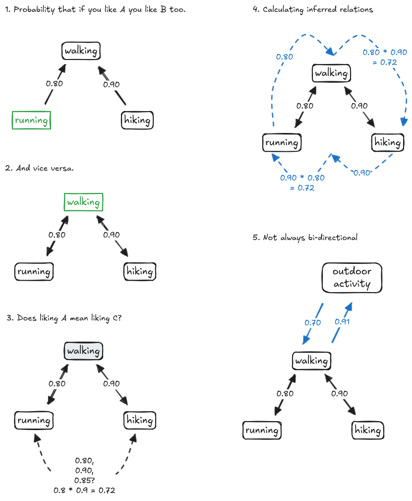
But wait, if I like hiking, am I likely to like running? There’s no arrow between those, and our graph implies there’s a relationship there, but we don’t know that we can safely infer such things. Plus, should we be conservative and say it’s 80% likely or should we be optimistic and say 90%, or average the two at 85%? We might even be more conservative and “walk the graph” and multiply .8 * .9 to get 72% likelihood (See picture 3 and 4). Plus, we know that this isn’t purely bidirectional, so someone who said they like “outdoor activities” might also like walking 70% of the time, but someone who likes walking may be 91% likely to like “outdoor activities”…

For fun here’s some naive code. We can imagine inferring a few hops, reviewing dijkstra’s algo, etc.

graph = {
    ("running", "walking"): 0.80, ("walking", "running"): 0.80,
    ("hiking", "walking"): 0.90, ("walking", "hiking"): 0.90,
}

def score(a, b):
    if (a, b) in graph:
        return "direct", f"{graph[(a, b)]:.4f}"
    
    shared = [x for x in ["running", "hiking", "walking"] if (a, x) in graph]
    if shared:
        return "one-hop", f"{graph[(a, shared[0])] * graph[(shared[0], b)]:.4f}"
    return "no path", 0

print("running → walking:", score("running", "walking"))
print("hiking → walking:", score("hiking", "walking"))

print("running → hiking:", score("running", "hiking"))

running → walking: ('direct', '0.8000')
hiking → walking: ('direct', '0.9000')
running → hiking: ('one-hop', '0.7200')

Of course, it’s great if we can enumerate the nodes we need in the graph, but often there are too many terms we might not know. Consider that someone may say “I like running” or “I’m a runner” or “I go for runs” and simply searching for “running” as an interest will miss 2 terms out of three of these. Stemming and other tricks might help but they’re brittle. We always come across data we didn’t expect, e.g. we might read “I was a sprinter on the track team” or “I like sprinting” and miss that they have an interest in “running”.

A newer way to look at this problem is to leverage ML. LLMs are great at exactly this kind of problem. For an application we may not want to use a full prompt and LLM API call, but luckily we can use embeddings and vectorDBs to help. Let’s quickly look at the word embeddings for walk, run, hike and see what we get in terms of cosine distances:

import chromadb
from chromadb.utils import embedding_functions
import numpy as np


def main():
    embedding_fn = embedding_functions.SentenceTransformerEmbeddingFunction(
        model_name="average_word_embeddings_glove.6B.300d"  # Word-optimized model
    )
    data = ["walk", "run", "hike"]
    embeddings = embedding_fn(data)
    print(f"Embedding vector eg: sz={len(embeddings[0])}, looks like: {embeddings[0][:5]}...")
    print("Pairwise cosine similarities (0-1, 1.0=same):")
    for i in range(len(data)):
        for j in range(i + 1, len(data)):
            sim = cosine_similarity(embeddings[i], embeddings[j])
            print(f"* {data[i]:>6} <-> {data[j]:<6}: {sim:.4f}")


def cosine_similarity(vec1, vec2):
    dot_product = np.dot(vec1, vec2)
    norm_product = np.linalg.norm(vec1) * np.linalg.norm(vec2)
    return dot_product / norm_product


if __name__ == "__main__":
    main()

Embedding vector eg: sz=300, looks like: [-0.014619 -0.17277  -0.11171   0.31864  -0.52504 ]...
Pairwise cosine similarities (0-1, 1.0=same):
*   walk <-> run   : 0.4750
*   walk <-> hike  : 0.3058
*    run <-> hike  : 0.2077

Interesting:. This model finds walk and run to be the most similar, walk and hike the next, and hike and run the least similar

Today, we have embeddings, which give us a nice calculation of “conceptual distance”. What this means is we can get these “relationship” numbers “for free” without necessarily building this graph out. Plus vectorDBs are amazing at quickly giving us the top-K of similar items. Embedding models have done the work of figuring out, across huge corpuses of text, what these words and concepts mean, especially in relation to each other. And that’s probably good enough for a lot of use cases.

There’s a caveat here, which is to say that words without context can be dangerous. I worked in web search and we used to say “Fencing can be a sport, the stuff that borders your house, or what you do with stolen goods”. So, depending on your embedding model, you may want to calculate from full sentences such as “I like the activity walking” and “I like the activity running” as opposed to using the bare words.

A quick change to the more popular Sentence model “all-MiniLLM-L6-v2”:

    embedding_fn = embedding_functions.SentenceTransformerEmbeddingFunction(
        model_name="all-MiniLM-L6-v2"  # Sentence transformer model
    )
    data = ["I like to walk", "I like to run", "I like to hike"]
    embeddings = embedding_fn(data[:3])

Embedding vector eg: sz=384, looks like: [-0.06094085 -0.05805941  0.03494389  0.09246249  0.0638584 ]...
Pairwise cosine similarities (0-1, 1.0=same):
* I like to walk <-> I like to run: 0.6254
* I like to walk <-> I like to hike: 0.7236
* I like to run <-> I like to hike: 0.5118

Interesting. This model has a different perspective, which could be the model or the context of interests and preferences (or both).

The most powerful and robust feature here is that we can handle almost any input without the need to pre-calculate our graph and weights. If we have an enumeration of categories of people’s favorite activities, and we see an event category that’s new to us, we can make an educated guess about how to map them, or use the embedding as input to our ranking. Meaning, if we put event descriptions into our vectorDB, then search for “I like to walk”, then a hiking event should score well.

Of course, a combination of the two concepts would be needed in a real system since “interests” isn’t the same as “semantic meaning”. Here we controlled the sentence, but if you put in “I hate to walk” it turns out that sentence scores 0.7697 from “I like to walk” because these are close in latent space although one part of the vector is pointing in the opposite direction. If you can afford the latency of calling a foundational LLM with a prompt, it would handle such a case nicely.

My friend is still playing around with his code, but running through these ideas gave him some fun approaches to think about. Matching, recommendation systems, and ranking are always interesting to play with and there’s always more to explore.

What’s your experience on these topics? Feel free to ask questions in the comments, or let me know what other topics you’d like to know about. I always monitor them for awhile after publishing.

End Notes:

#

• Production quality is all about the details, so you should always test and benchmark. A vectorDB search is fast, but if you need accuracy and control then the right approach may be building a graph and calculating these weights yourself (doing several queries to get answers).
• At the time of writing, Weaviate was the only vectorDB I found that directly supports graphDB features.
• We used a couple models, so beware that the embedding vectors between them are not compatible. e.g. never compare vectors from a word model against a sentence model.

Thanks Richard King for the fencing examples ;-)